The visualization gallery • msuiter

Every plotting face of the package on one page, organized by the question each figure answers. One small simulated cohort drives the whole gallery: the setup block draws it with ms_simulate(), then runs the fast faces – ms_fit() for reference exposures, ms_extract() for de-novo signatures, plus the bootstrap, stratification, embedding and QC surfaces – so every figure below reuses the same MsCatalog, MsSignature and MsFit objects. The variant-to-catalog face (ms_tally()) is not needed here; it is covered in get-started.html. Each example opens with the situation the figure is for; all faces return ggplot objects, so anything shown can be re-themed or extended with the usual ggplot2 layers.

One cohort for the whole gallery

The dictionary is sliced from the bundled COSMIC reference face, whose matrices already carry the canonical SBS96 channel labels.

refdb <- ms_refdb_bundled(build = "GRCh38")
#> ms_refdb_bundled: no official ID reference set for build GRCh38 -- serving the declared build-independent set (nearest official build(s): GRCh37)
sbs <- refdb[["SBS_GRCh38"]]@matrices[[1]]
dict <- sbs[, c("SBS1", "SBS5", "SBS13", "SBS57")]

The cohort plants a clock-like pair everywhere, an APOBEC signature in a subgroup, the artifact signature SBS57 in another subgroup, and one deliberately hypermutated member that rides a count-scale exposure column instead of a share column.

samples <- c(paste0("T", 1:12), "H1")
act <- matrix(0, nrow = ncol(dict), ncol = length(samples),
              dimnames = list(colnames(dict), samples))
act["SBS1", samples[1:12]] <- 0.50
act["SBS5", samples[1:12]] <- 0.42
act["SBS13", c("T1", "T2", "T3", "T4")] <- 0.08
act["SBS57", c("T5", "T6")] <- 0.08
resid <- 1 - colSums(act[, samples[1:12]])
act["SBS1", samples[1:12]] <- act["SBS1", samples[1:12]] + resid / 2
act["SBS5", samples[1:12]] <- act["SBS5", samples[1:12]] + resid / 2
act["SBS1", "H1"] <- 12500
act["SBS5", "H1"] <- 10000
act["SBS13", "H1"] <- 2500
cat <- ms_simulate(dict, act, burden = 600, seed = 14)
cat
#> <MsCatalog> SBS96: 96 channels x 13 samples

The reused objects, all at minimal settings so the page renders quickly (the de-novo face uses a single seeded NMF engine; ms_extract()’s default consensus pipeline and the bootstrap’s default replicate count are the thorough settings for real analyses).

fit <- ms_fit(cat, dict)
sig <- ms_extract(cat, k = 3, method = "nmf")
boot <- ms_fit_bootstrap(cat, dict, method = "nnls", n_boot = 50, seed = 1,
                         return_draws = TRUE)
strat <- ms_stratify_hypermutants(cat, seed = 1)
emb <- ms_embed(fit@exposures, method = "kmeans", clusters = 2L, seed = 1)
qc <- ms_qc_report(cat, dict, fit@exposures)
roster <- ms_qc_roster_share(cat, dict, fit@exposures)

Catalog and signature profiles

plot_catalog_profile() is for rendering a single profile column – one catalog sample or one signature – in the COSMIC bar style, with the substitution classes colored and the flanking-context labels vertical.

plot_catalog_profile(cat@counts, column = "T1")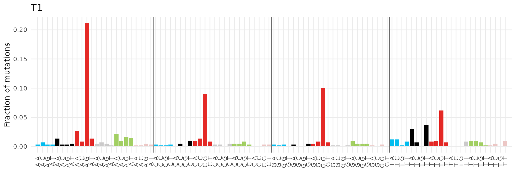

In mode = "count" the y axis carries raw mutations instead of shares – the natural reading for a burden outlier such as the hypermutated member.

plot_catalog_profile(cat@counts, column = "H1", mode = "count")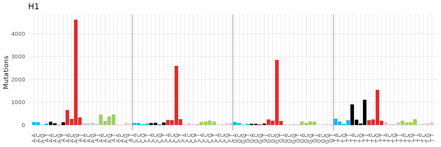

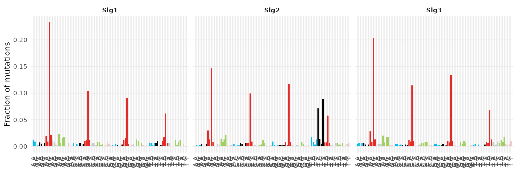
plot_signature_catalog() is for inspecting a whole signature set at once: the same semantics, one panel per signature. It accepts a matrix or an MsSignature directly.

plot_signature_catalog(sig)

Reference comparison

plot_cosmic_scatter() is for judging, channel by channel, how an estimated profile lines up against a reference profile: the identity line, the cosine, and an empirical signature-null tail probability are annotated on the plot itself.

plot_cosmic_scatter(sig@signatures[, 1], dict[, "SBS1"], label = "SBS1")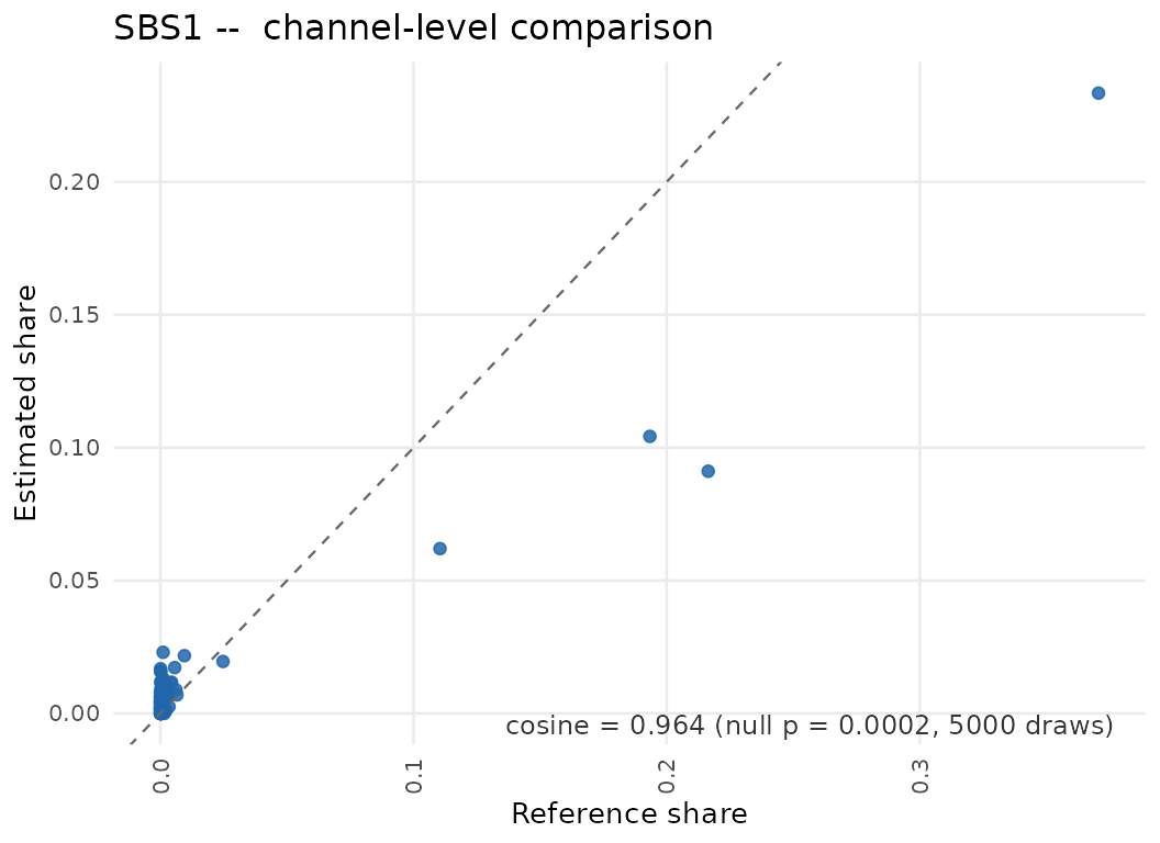

plot_reference_comparison() is for the same pairing when the deviations matter more than the summary: the estimate is drawn dark and the reference light, on shared axes.

plot_reference_comparison(sig@signatures[, 1], dict[, "SBS1"])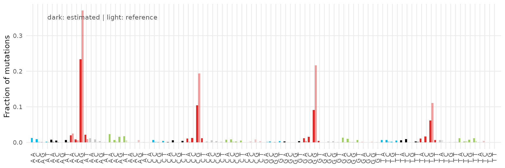

Exposure structure

plot_exposure_heatmap() is for reading the cohort-wide exposure matrix at a glance, one row per sample; the exposure faces accept the labelled matrix or an MsSignature.

plot_exposure_heatmap(fit@exposures)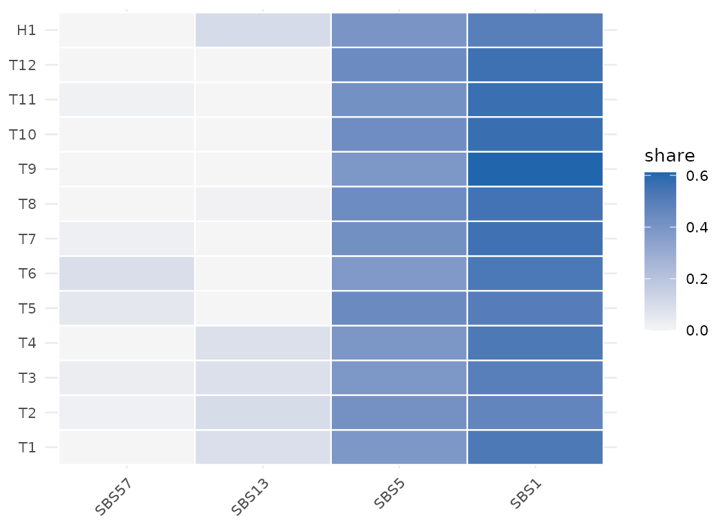

plot_exposure_stacked() is for the compositional story per sample: one bar per sample, stacked by signature share.

plot_exposure_stacked(fit@exposures)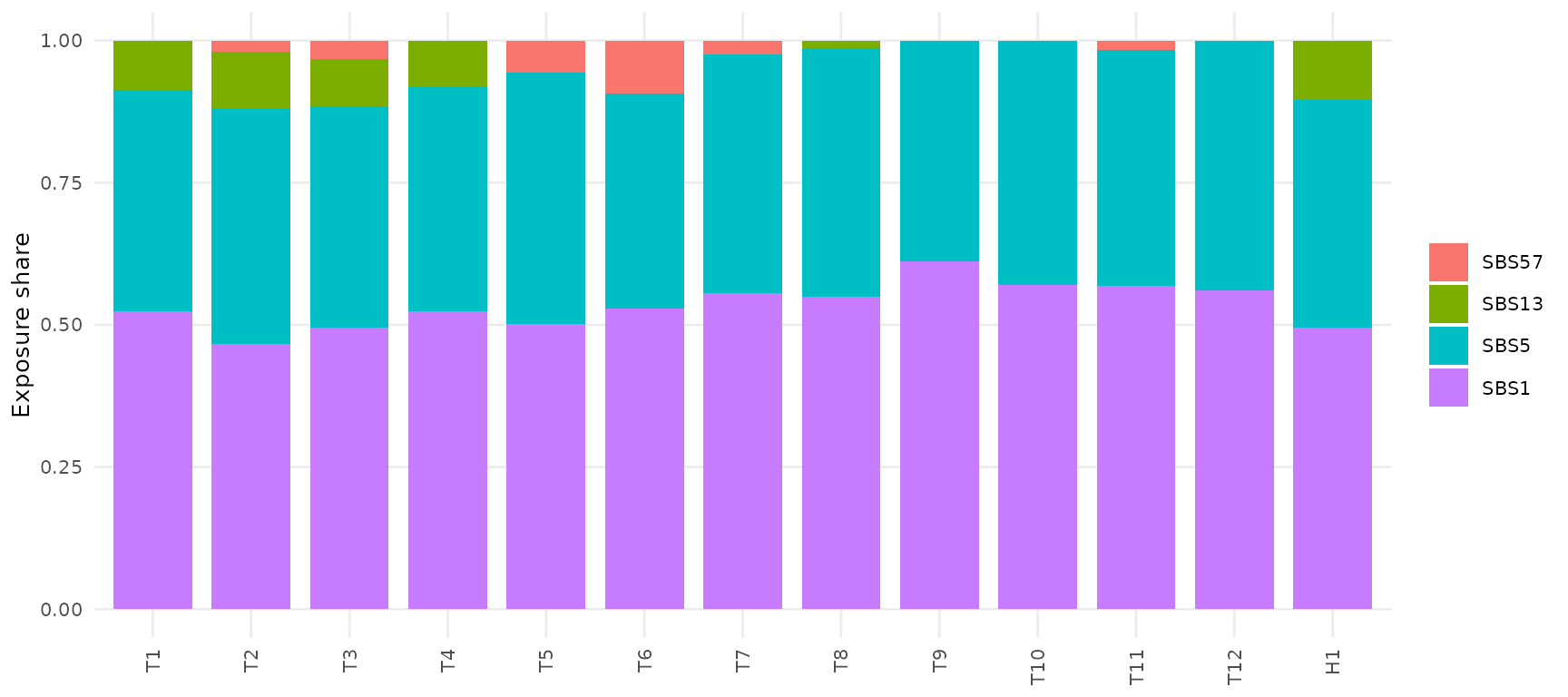

plot_exposure_riverplot() is for the same table read as flows between the sample axis and the signature axis (requires the ggalluvial package).

plot_exposure_riverplot(fit@exposures)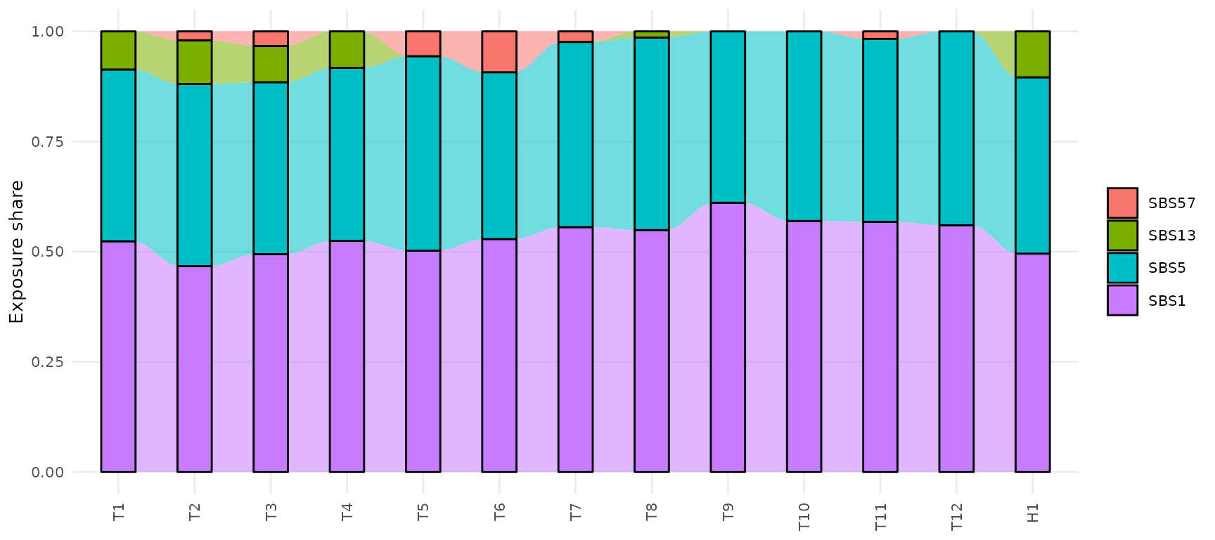

Evidence panels

plot_boot_ci() is for a single sample’s decomposition with uncertainty bars: point exposures with their bootstrap percentile whiskers, ordered by exposure share.

plot_boot_ci(boot, sample = "H1")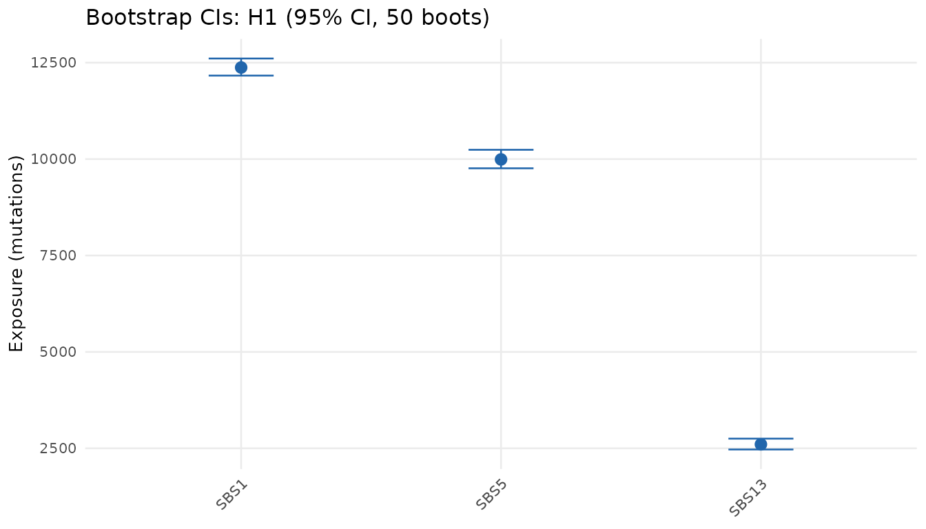

plot_boot_distribution() is for the shape of the resampling evidence itself, not just the interval endpoints: per-signature histograms of the raw boot draws, with the estimate and both bounds marked (the fit must carry the draws cube, hence return_draws = TRUE above).

plot_boot_distribution(boot, sample = "T1")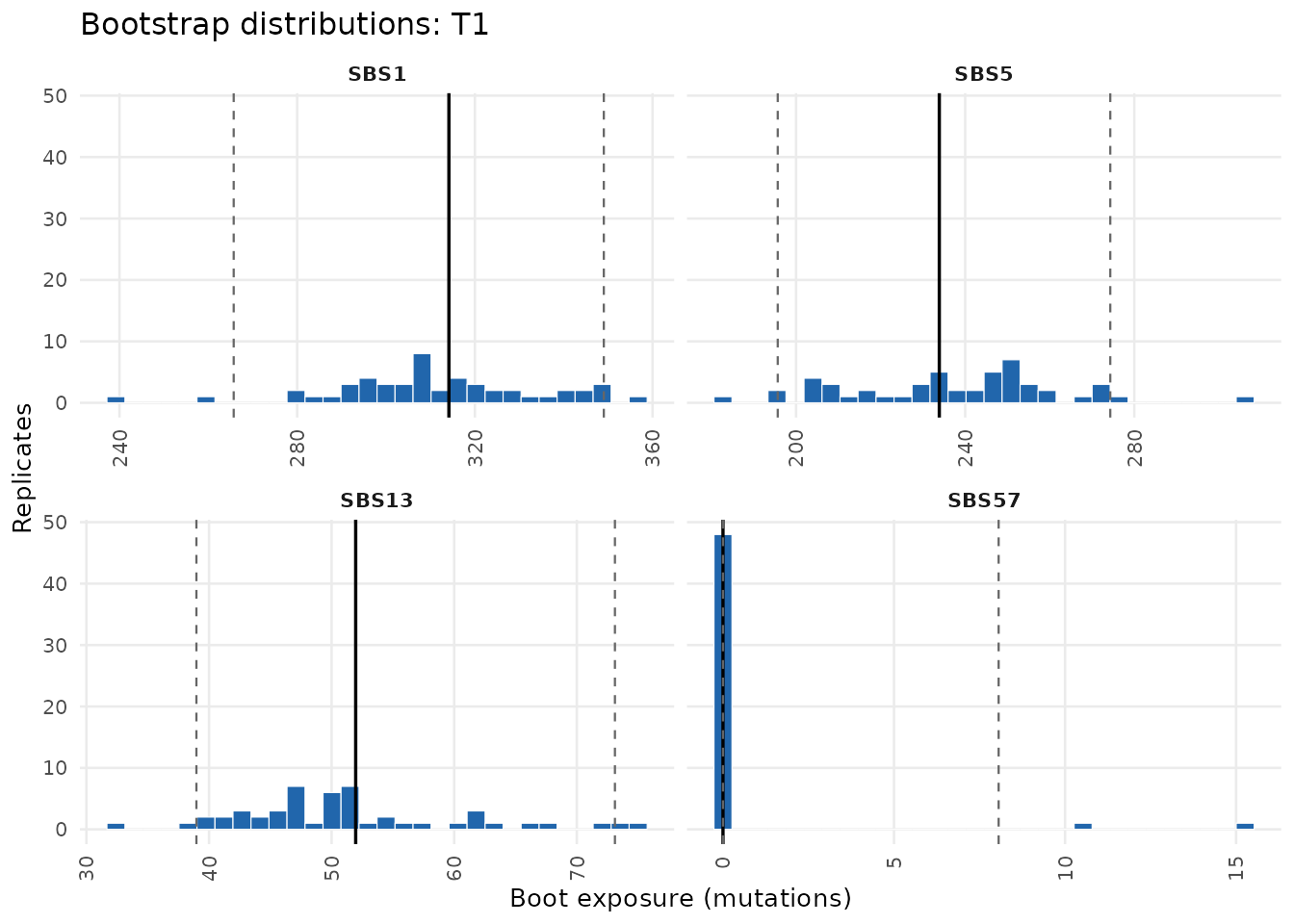

plot_hypermutator_burden() is for seeing who was flagged as hypermutated: a burden histogram colored by the stored adjudication, with the stored cutoff as a dashed line – nothing is re-thresholded at plot time.

plot_hypermutator_burden(strat)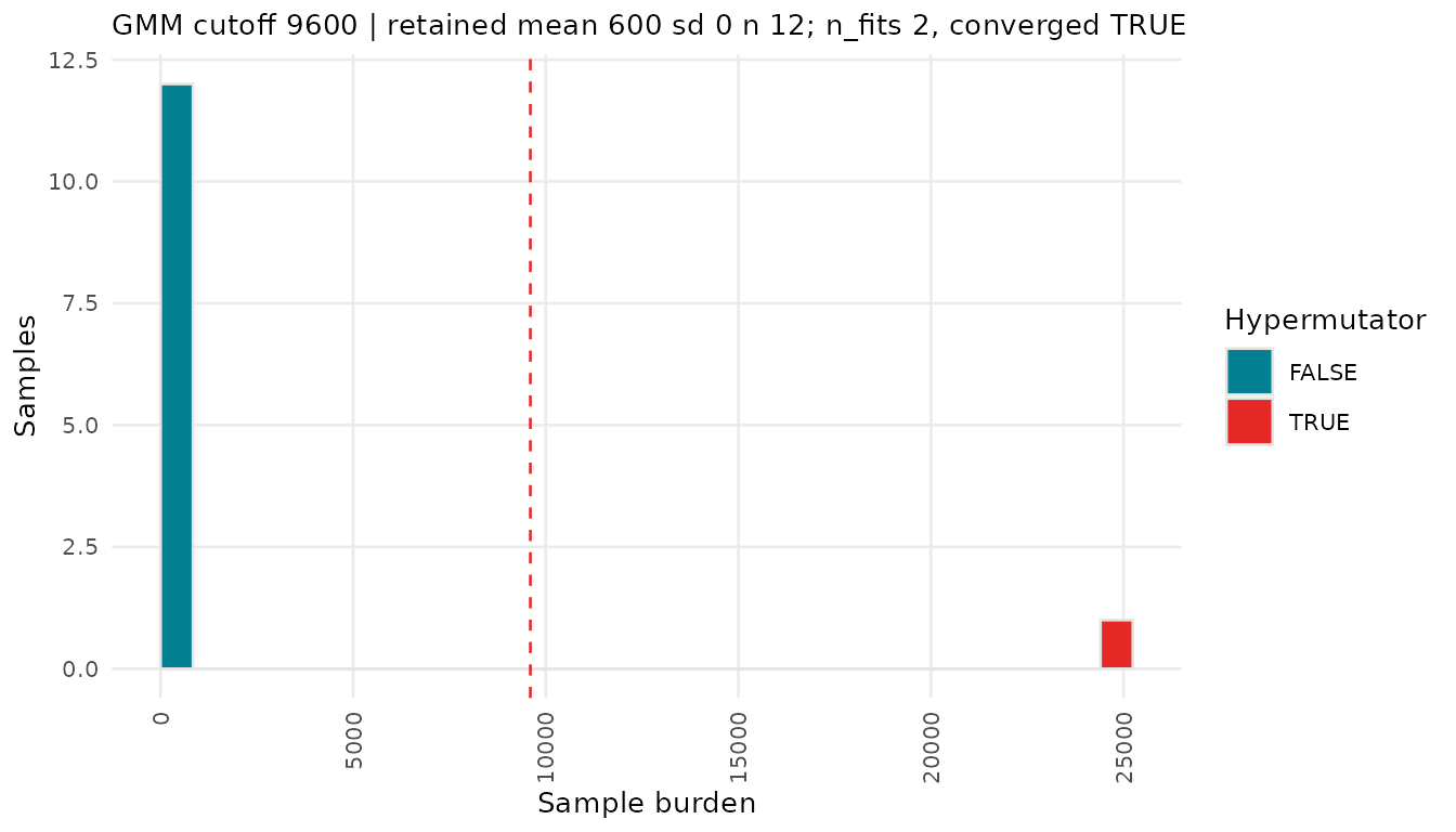

plot_embedding() is for seeing how samples organize in exposure space; when the embedding table carries a cluster column the points are colored by it.

plot_embedding(emb)
#> Ignoring unknown labels:
#> • colour : "cluster"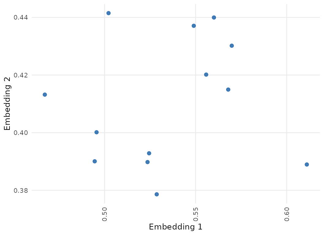

QC

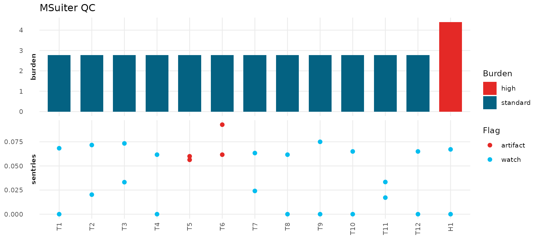
plot_qc_dashboard() is for reading per-sample burden and the artifact sentries on one shared sample axis, drawn exactly as the QC report stored them – burden classes on the top panel, the G>T and C>T sentinel shares below, colored by the stored flags.

plot_qc_dashboard(qc)

plot_pseudosig_contribution() is for ranking the per-sample artifact share of the exposure, with the contributing artifact signatures labelled and the flagged samples colored by their verdict.

plot_pseudosig_contribution(roster)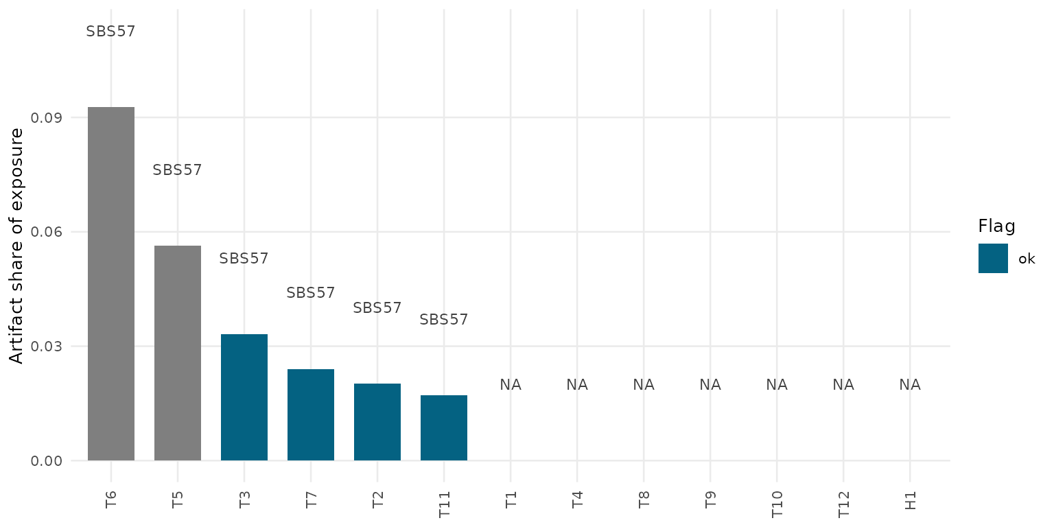

Where to go next

The figures above draw what the certified faces stored; the statistics behind the comparison machinery are the subject of Comparing signatures, and the QC surfaces themselves – the report, the roster share and their flags – are documented in Quality control.