Fitting known signatures: exposures, presence tests, and bootstrap intervals • msuiter

De-novo extraction (ms_extract()) discovers signatures; reference fitting answers the mirror-image question. Given a trusted signature dictionary, ms_fit() estimates each sample’s exposure to every dictionary signature, ms_test_presence() asks which signatures the cohort’s evidence supports at all, and ms_fit_bootstrap() attaches bootstrap confidence intervals and support stability to the same fit. This guide walks the three faces on one small simulated cohort, then reads the MsFit result object and the bootstrap plotting faces. The upstream steps (variants, tallying) are covered in get-started.html.

A simulated cohort against COSMIC signatures

The dictionary is a channels x signatures matrix, or an MsSignature whose signatures matrix is used. The bundled COSMIC reference database ships canonical SBS96 matrices whose rows already carry the canonical channel labels, so slicing a few columns gives a dictionary that ms_fit() can align by label.

refdb <- ms_refdb_bundled(build = "GRCh38")
#> ms_refdb_bundled: no official ID reference set for build GRCh38 -- serving the declared build-independent set (nearest official build(s): GRCh37)
sbs <- refdb[["SBS_GRCh38"]]@matrices[[1]]
dict <- sbs[, c("SBS1", "SBS5", "SBS13", "SBS4")]
dim(dict)
#> [1] 96  4

A subgroup of samples plants an APOBEC signature on top of the clock-like pair; another dictionary signature is planted nowhere, so the presence test below has something to reject.

samples <- paste0("T", 1:12)
act <- matrix(0, nrow = ncol(dict), ncol = length(samples),
              dimnames = list(colnames(dict), samples))
act["SBS1", ] <- 0.45
act["SBS5", ] <- 0.45
act["SBS13", samples[1:4]] <- 0.10
# share exposures: rebalance the clock pair so every column sums to one
resid <- 1 - colSums(act)
act["SBS1", ] <- act["SBS1", ] + resid / 2
act["SBS5", ] <- act["SBS5", ] + resid / 2
cat <- ms_simulate(dict, act, arm = "multinomial", burden = 600, seed = 11)
cat
#> <MsCatalog> SBS96: 96 channels x 12 samples

ms_simulate() returns an MsCatalog, exactly the input ms_fit() dispatches on.

Fitting exposures with ms_fit()

The default method, "nnls", solves the Lawson-Hanson non-negative least squares problem per sample: the classical deconstructSigs-style baseline. The other two methods start from that solution and refine it on a likelihood scale:

"likelihood_bidirectional" (MuSiCal flavour) alternates backward and forward steps on the per-mutation multinomial log-likelihood: a signature leaves when the cheapest removal costs less than the epsilon threshold and enters when the best gain exceeds it, until both steps decline;
"lrt" (mSigAct flavour) maximizes the negative-binomial likelihood over the exposures through an internal safeguarded-Newton ascent, warm-started from NNLS.

fit <- ms_fit(cat, dict) # method = "nnls" (default)
fit
#> <MsFit> 4 signatures x 12 samples | engine: nnls | refdb: adhoc-1
head(fit@support)
#>   signature sample exposure     share active
#> 1      SBS1     T1 269.1006 0.4485010   TRUE
#> 2      SBS5     T1 257.2659 0.4287765   TRUE
#> 3     SBS13     T1  73.6335 0.1227225   TRUE
#> 4      SBS4     T1   0.0000 0.0000000  FALSE
#> 5      SBS1     T2 248.8291 0.4154832   TRUE
#> 6      SBS5     T2 282.0921 0.4710242   TRUE
head(fit@tests)
#>   signature sample  lrt_stat         lrt_p        se
#> 1      SBS1     T1 384.21030  7.538704e-86 17.775025
#> 2      SBS5     T1 495.11013 5.506652e-110 18.191517
#> 3     SBS13     T1  83.40555  3.341701e-20  9.877928
#> 4      SBS4     T1   0.00000  5.000000e-01        NA
#> 5      SBS1     T2 333.73923  7.368207e-75 17.197792
#> 6      SBS5     T2 282.16723  1.265599e-63 18.883105

Two tidy evidence tables ride along. support holds one row per signature-sample pair with the exposure, its compositional share and the zeroing decision: exposures whose share falls below zero_threshold are set to exactly zero and reported active = FALSE. tests holds the entry-wise presence LRT statistic and raw p-value per pair, plus a Fisher standard error that exists only on the interior support – boundary parameters get tests, not intervals, so boundary rows carry NA.

Two further arguments shape the whole fit. rescale = TRUE (default) multiplies each sample’s kept exposures back onto the sample’s original mutation total, the MuSiCal TMB-rescale semantics: the multiplication leaves zeroed entries at zero, and the shares (hence the zeroing decision) and the presence evidence are invariant. connected = NULL by default; passing distinct dictionary column indices selects a connected-signature group – for example the clock-like background pair – which is fixed at its initial full-NNLS solution after the method refit (FixAndRefit) while the remaining signatures are re-optimized against the residual. This is a documented approximation of the upstream joint-refit strategy, which is declared future work and never silently substituted.

Choosing among the methods

All three methods run through the same kernel, and the tests evidence is method-independent by construction: the LRT columns are always computed at the negative-binomial MLE exposures, so the tables compare fairly across methods. The nb_size argument is the negative-binomial size of every likelihood-based column; larger values sit closer to the Poisson limit.

fits <- list(
  nnls = fit,
  bidirectional = ms_fit(cat, dict, method = "likelihood_bidirectional"),
  lrt = ms_fit(cat, dict, method = "lrt")
)
round(vapply(fits, function(f) f@exposures[, "T1"], numeric(ncol(dict))), 1)
#>        nnls bidirectional   lrt
#> SBS1  269.1         269.1 269.1
#> SBS5  257.3         257.3 257.3
#> SBS13  73.6          73.6  73.6
#> SBS4    0.0           0.0   0.0

Testing cohort presence with ms_test_presence()

ms_test_presence() tests, per signature, whether the signature is present in the cohort. Per-sample entry-wise LRT statistics are pooled by summation (independent likelihoods add), and the raw p-value is the exact pooled-null tail: under the null each per-sample statistic follows the Self-Liang boundary law (an equal mixture of a point mass at zero and a chi-square), so the pooled statistic over independent samples is a Binomial-weighted mixture of chi-squares. Benjamini-Hochberg correction runs over the signature family, and pass_bh applies the frozen family-wise alpha.

ms_test_presence(cat, dict) # kernel face: catalog + dictionary
#>   signature        stat        p_raw         p_bh pass_bh
#> 1      SBS1 4478.368208 0.000000e+00 0.000000e+00    TRUE
#> 2      SBS5 9420.543645 0.000000e+00 0.000000e+00    TRUE
#> 3     SBS13  316.849472 2.266357e-63 3.021809e-63    TRUE
#> 4      SBS4    5.304463 4.961519e-01 4.961519e-01   FALSE
ms_test_presence(fit)       # MsFit face: re-aggregates the fit's own evidence
#>   signature        stat        p_raw         p_bh pass_bh
#> 1      SBS1 4478.368208 0.000000e+00 0.000000e+00    TRUE
#> 2      SBS5 9420.543645 0.000000e+00 0.000000e+00    TRUE
#> 3     SBS13  316.849472 2.266357e-63 3.021809e-63    TRUE
#> 4      SBS4    5.304463 4.961519e-01 4.961519e-01   FALSE

The result is a plain data.frame with one row per dictionary signature, so it drops into any downstream filter or report. The two faces agree by construction – the MsFit face re-derives its p-values from the fit’s stored evidence grid with the pure-R twin of the kernel’s arithmetic.

Bootstrap intervals and stability with ms_fit_bootstrap()

The bootstrap resamples each sample’s mutations from its empirical channel distribution (nonparametric multinomial), refits the selected method per replicate, and reports the percentile interval over the replicate exposures plus the support stability – the frequency with which the zeroing rule keeps each exposure active. The result is an MsFit like ms_fit() returns, enriched with attributes on the exposures matrix; the support table gains a boot_stability column. The point exposures and tests remain an ordinary point fit: the interval is support-conditional evidence alongside the LRT, not a replacement for it. With return_draws = TRUE the raw per-replicate exposure cube is attached as the boot_draws attribute for the histogram face below; bca = TRUE adds the bias-corrected-and-accelerated interval computed from the same replicates. The default replicate count is higher; this guide keeps n_boot small for rendering speed.

boot <- ms_fit_bootstrap(cat, dict, method = "nnls", n_boot = 50, seed = 1,
                         return_draws = TRUE)
boot
#> <MsFit> 4 signatures x 12 samples | engine: nnls | refdb: adhoc-1
head(boot@support)
#>   signature sample exposure     share active boot_stability
#> 1      SBS1     T1 269.1006 0.4485010   TRUE              1
#> 2      SBS5     T1 257.2659 0.4287765   TRUE              1
#> 3     SBS13     T1  73.6335 0.1227225   TRUE              1
#> 4      SBS4     T1   0.0000 0.0000000  FALSE              0
#> 5      SBS1     T2 248.8291 0.4154832   TRUE              1
#> 6      SBS5     T2 282.0921 0.4710242   TRUE              1
names(attributes(boot@exposures))
#> [1] "dim"               "dimnames"          "ci_lower"         
#> [4] "ci_upper"          "support_stability" "n_boot"           
#> [7] "seed"              "ci_level"          "boot_draws"
dim(attr(boot@exposures, "boot_draws"))
#> [1]  4 12 50

The CI endpoints are labelled matrices with the same shape as the exposures, so the interval for one sample reads directly as a table.

round(cbind(lower = attr(boot@exposures, "ci_lower")[, "T1"],
            estimate = boot@exposures[, "T1"],
            upper = attr(boot@exposures, "ci_upper")[, "T1"],
            stability = attr(boot@exposures, "support_stability")[, "T1"]), 1)
#>       lower estimate upper stability
#> SBS1  241.7    269.1 292.7         1
#> SBS5  231.1    257.3 292.5         1
#> SBS13  52.4     73.6  97.1         1
#> SBS4    0.0      0.0   0.0         0

The MsFit object and the bootstrap plots

The MsFit container carries the labelled exposures matrix (signatures x samples), the support and tests data.frames, an adhoc reference_summary snapshot derived from the dictionary’s signature labels (a sha256 digest over the labels, never an embedded reference database), and the engine string recording the method. print shows one line with dimensions, engine and snapshot version; the plotting faces read the bootstrap attributes directly.

plot_boot_ci(boot, sample = "T1")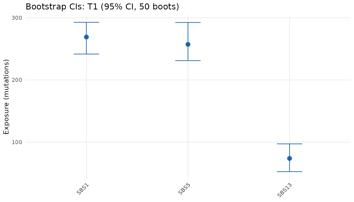

plot_boot_distribution(boot, sample = "T1") # requires return_draws = TRUE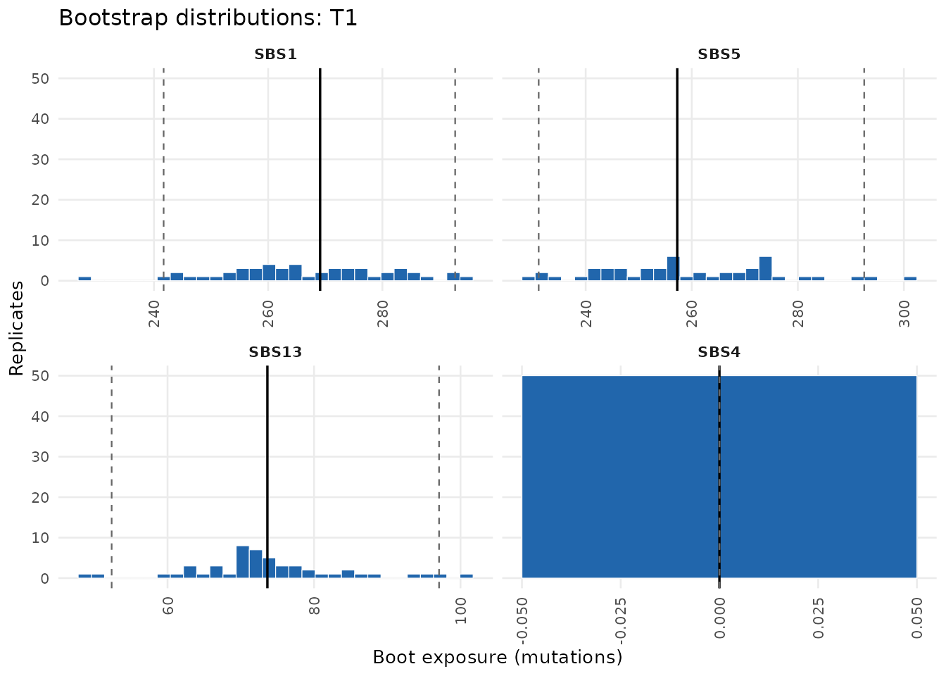

plot_boot_stability(boot, sample = "T1")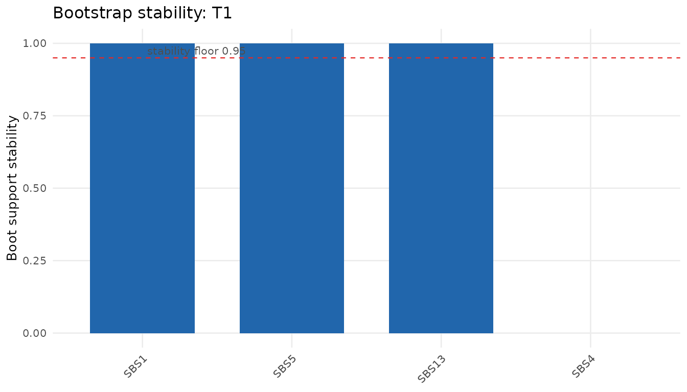

plot_boot_ci() draws the point exposures with their percentile whiskers for one sample, ordered by exposure share; plot_boot_distribution() shows the raw per-replicate exposure histograms with the estimate and both bounds marked; plot_boot_stability() bars the support stability against the calibration floor. Without the draws cube the histogram face raises a structured error that says to re-run ms_fit_bootstrap() with return_draws = TRUE.

Where to go next

Once signatures are fitted and their presence established, the natural next steps are comparing dictionaries and extracted catalogs – Comparing signatures – and the calibration statistics behind the presence and interval machinery – Calibrated statistics. The input path from VCFs to catalogs is in get-started.html.