Quickly Analyze Cancer Data with Data from UCSCXenaShiny

Shixiang Wang

Central South University
wangshx@csu.edu.cn

2025-08-10

library(bregr)
#> Welcome to 'bregr' package!
#> =======================================================================
#> You are using bregr version 1.1.0.9000
#> 
#> Project home : https://github.com/WangLabCSU/bregr
#> Documentation: https://wanglabcsu.github.io/bregr/
#> Cite as      : arXiv:2110.14232
#> =======================================================================
#> 
library(dplyr)
#> 
#> Attaching package: 'dplyr'
#> The following objects are masked from 'package:stats':
#> 
#>     filter, lag
#> The following objects are masked from 'package:base':
#> 
#>     intersect, setdiff, setequal, union

if (!requireNamespace("UCSCXenaShiny")) {
  install.packages("UCSCXenaShiny")
}
#> Loading required namespace: UCSCXenaShiny
library(UCSCXenaShiny)
#> =========================================================================================
#> UCSCXenaShiny version 2.2.0
#> Project URL: https://github.com/openbiox/UCSCXenaShiny
#> Usages: https://openbiox.github.io/UCSCXenaShiny/
#> 
#> If you use it in published research, please cite:
#>   Shensuo Li, Yuzhong Peng, Minjun Chen, Yankun Zhao, Yi Xiong, Jianfeng Li, Peng Luo, 
#>   Haitao Wang, Fei Zhao, Qi Zhao, Yanru Cui, Sujun Chen, Jian-Guo Zhou, Shixiang Wang,  
#>   Facilitating integrative and personalized oncology omics analysis with UCSCXenaShiny, 
#>   Communications Biology, 1200 (2024),  https://doi.org/10.1038/s42003-024-06891-2
#> =========================================================================================
#>                               --Enjoy it--

UCSCXenaShiny offers extensive builtin cancer datasets and data query functions to facilitate analysis and visualization.

Obtain Data

data <- inner_join(
  tcga_clinical_fine,
  tcga_surv |> select(sample, OS, OS.time),
  by = c("Sample" = "sample")
) |> filter(!is.na(Stage_ajcc), !is.na(Gender))
head(data)
#> # A tibble: 6 × 10
#>   Sample Cancer   Age Code  Gender Stage_ajcc Stage_clinical Grade    OS OS.time
#>   <chr>  <chr>  <dbl> <chr> <chr>  <chr>      <chr>          <chr> <dbl>   <dbl>
#> 1 TCGA-… ACC       58 TP    MALE   Stage II   NA             NA        1    1355
#> 2 TCGA-… ACC       44 TP    FEMALE Stage IV   NA             NA        1    1677
#> 3 TCGA-… ACC       23 TP    FEMALE Stage III  NA             NA        0    2091
#> 4 TCGA-… ACC       30 TP    MALE   Stage III  NA             NA        1     365
#> 5 TCGA-… ACC       29 TP    FEMALE Stage II   NA             NA        0    2703
#> 6 TCGA-… ACC       30 TP    FEMALE Stage III  NA             NA        1     490

Execute bregr Pipeline

Assessing the influence of AJCC Stage on overall survival can be done by analyzing data grouped by gender.

m <- br_pipeline(
  data = data,
  y = c("OS.time", "OS"),
  x = "Stage_ajcc", x2 = "Age",
  group_by = "Gender",
  method = "coxph"
)
#> exponentiate estimates of model(s) constructed from coxph method
#> at default
m
#> an object of <breg> class with slots:
#> • y (response variable): OS.time and OS
#> • x (focal term): Stage_ajcc
#> • x2 (control term): Age
#> • group_by: Gender
#> • data: <tibble[,11]>
#> • config: <list: method = "coxph", extra = "">
#> • models: <list: FEMALE_Stage_ajcc = <coxph>, MALE_Stage_ajcc = <coxph>, and
#> All_Stage_ajcc = <coxph>>
#> • results: <tibble[,22]> with colnames Group_variable, Focal_variable, term,
#> variable, var_label, var_class, var_type, var_nlevels, contrasts,
#> contrasts_type, reference_row, label, n_obs, n_ind, n_event, exposure,
#> estimate, std.error, …, conf.low, and conf.high
#> • results_tidy: <tibble[,9]> with colnames Group_variable, Focal_variable,
#> term, estimate, std.error, statistic, p.value, conf.low, and conf.high
#> 
#> Focal term(s) are injected into the model one by one,
#> while control term(s) remain constant across all models in the batch.

br_get_results(m, tidy = TRUE) |>
  knitr::kable()

Group_variable	Focal_variable	term	estimate	std.error	statistic	p.value	conf.low	conf.high
FEMALE	Stage_ajcc	Stage_ajccStage II	1.273682	0.0959397	2.521499	0.0116856	1.055351	1.537181
FEMALE	Stage_ajcc	Stage_ajccStage III	2.149478	0.0967063	7.912875	0.0000000	1.778347	2.598062
FEMALE	Stage_ajcc	Stage_ajccStage IV	5.178744	0.1081300	15.209118	0.0000000	4.189710	6.401251
FEMALE	Stage_ajcc	Age	1.035787	0.0025991	13.528430	0.0000000	1.030524	1.041077
MALE	Stage_ajcc	Stage_ajccStage II	1.768884	0.0833656	6.841537	0.0000000	1.502237	2.082861
MALE	Stage_ajcc	Stage_ajccStage III	2.235855	0.0811756	9.912137	0.0000000	1.906983	2.621443
MALE	Stage_ajcc	Stage_ajccStage IV	3.379213	0.0849960	14.325886	0.0000000	2.860664	3.991759
MALE	Stage_ajcc	Age	1.029710	0.0023311	12.559176	0.0000000	1.025016	1.034425
All	Stage_ajcc	Stage_ajccStage II	1.468986	0.0628836	6.115624	0.0000000	1.298647	1.661668
All	Stage_ajcc	Stage_ajccStage III	2.193520	0.0621347	12.642015	0.0000000	1.942014	2.477597
All	Stage_ajcc	Stage_ajccStage IV	4.014838	0.0665694	20.880417	0.0000000	3.523741	4.574377
All	Stage_ajcc	Age	1.033083	0.0017248	18.869895	0.0000000	1.029596	1.036581

Generate Visualizations

For example:

m <- br_rename_models(m, c("Female", "Male", "All"))
#> rename model names from "FEMALE_Stage_ajcc", "MALE_Stage_ajcc", and
#> "All_Stage_ajcc" to "Female", "Male", and "All"

br_show_forest_ggstats(m)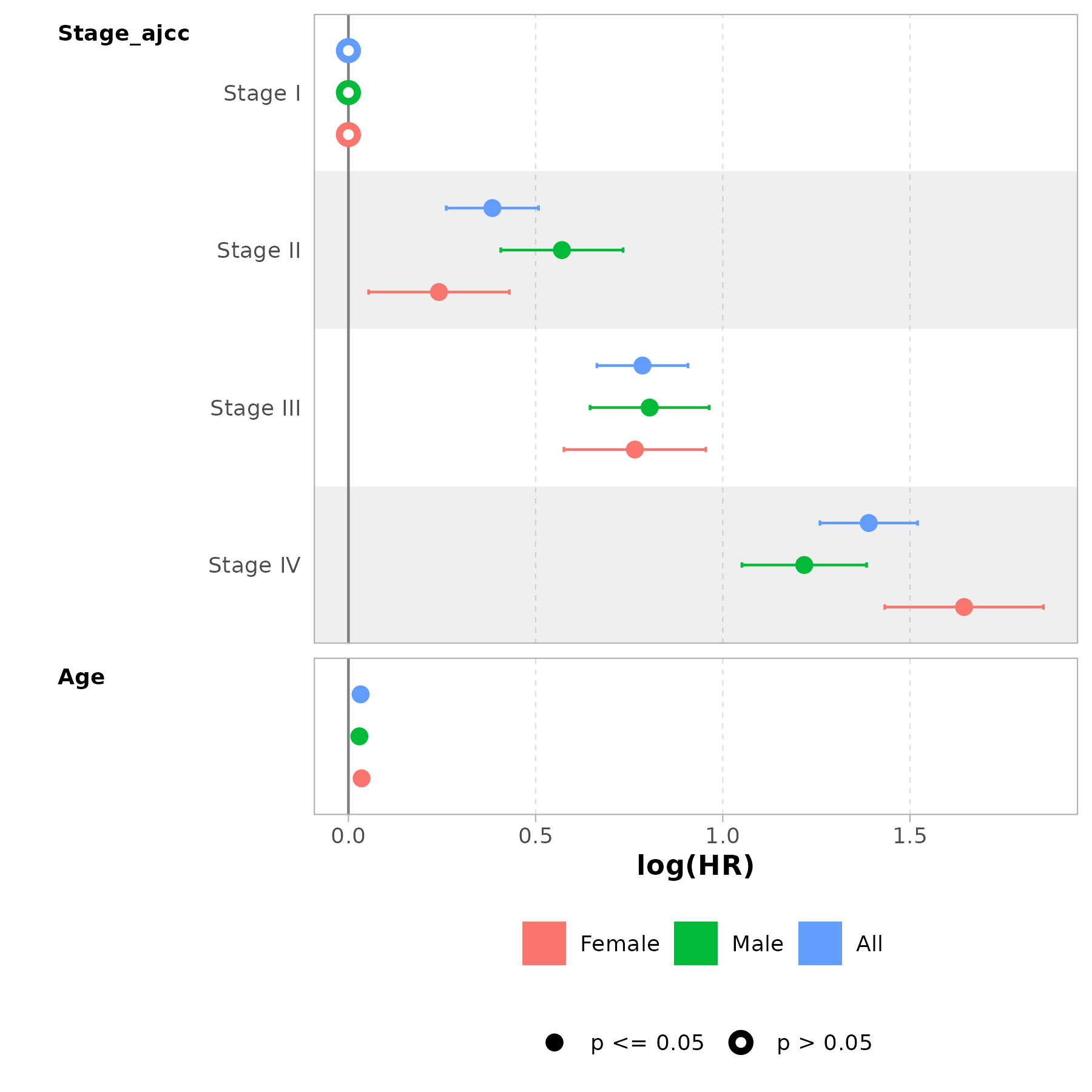

Explore Further

Besides, using tcga_surv_get(), you can efficiently retrieve values for a specified gene (c("mRNA", "miRNA", "methylation", "transcript", "protein", "mutation", "cnv")) from the TCGA cohort.

For more comprehensive guidance on querying various omics data from different databases/cohorts, refer to the Molecular Data Query section of the UCSCXenaShiny tutorial book.