R6 class representing a list of regression model

Contains fields storing data and methods to build, process and visualize a list of regression model (REGModel).

Public fields

data: A data.table storing modeling data.
x: Focal variables (terms).
y: Predicted variables or expression.
covars: Covariables.
group: A split variable.
mlist: A list of REGModel.
args: Other arguments used for building model.
type: Model type (class).
result: Model result, a object of parameters_model. Can be converted into data.frame with as.data.frame() or data.table::as.data.table().
forest_data: More detailed data used for plotting forest.

Methods

Method `new()`

Create a REGModelList object.

Usage

REGModelList$new(data, y, x, covars = NULL, group = NULL)

Arguments

data: A data.table storing modeling data.
y: Predicted variables or expression.
x: Focal variables (terms).
covars: Covariables.
group: A split variable.

Returns

A REGModelList R6 object.

Method `build()`

Build REGModelList object.

Usage

REGModelList$build(
  f = c("coxph", "binomial", "gaussian", "Gamma", "inverse.gaussian", "poisson", "quasi",
    "quasibinomial", "quasipoisson"),
  exp = NULL,
  ci = 0.95,
  parallel = FALSE,
  ...
)

Arguments

f: A length-1 string specifying modeling function or family of glm(), default is 'coxph'. Other options are members of GLM family, see stats::family(). 'binomial' is logistic, and 'gaussian' is linear.
exp: Logical, indicating whether or not to exponentiate the the coefficients.
ci: Confidence Interval (CI) level. Default to 0.95 (95%). e.g. survival::coxph().
parallel: If TRUE, use N-1 cores to run the task.
...: Other parameters passing to corresponding regression model function.

Returns

A REGModel R6 object.

Method `plot_forest()`

Plot forest.

Usage

REGModelList$plot_forest(
  ref_line = NULL,
  xlim = NULL,
  vars = NULL,
  p = NULL,
  ...
)

Arguments

ref_line: Reference line, default is 1 for HR.
xlim: Limits of x axis.
vars: Selected variables to show.
p: Selected variables with level' p value lower than p.
...: Other plot options passing to forestploter::forest(). Also check https://github.com/adayim/forestploter to see more complex adjustment of the result plot.

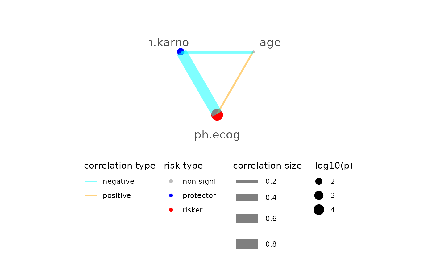
Method `plot_connected_risk()`

Plot connected risk network Append scale_size() operation (i.e.,scale_size(range = c(0.1, 4))) to reset the range of line width

Usage

REGModelList$plot_connected_risk()

Method `print()`

Print the REGModelList object

Usage

REGModelList$print(...)

Arguments

...: Unused.

Method `clone()`

The objects of this class are cloneable with this method.

Usage

REGModelList$clone(deep = FALSE)

Arguments

deep: Whether to make a deep clone.

Examples

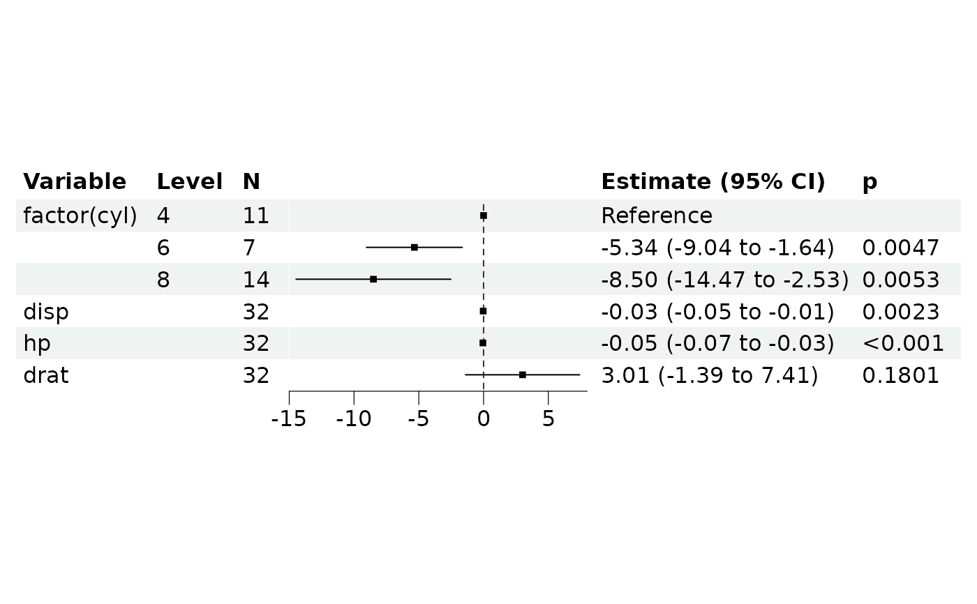
# GLM regression
ml <- REGModelList$new(
  data = mtcars,
  y = "mpg",
  x = c("factor(cyl)", colnames(mtcars)[3:5]),
  covars = c(colnames(mtcars)[8:9], "factor(gear)")
)
ml
#> <REGModelList>    ========== 
#> 
#> X(s): factor(cyl), disp, hp, drat 
#> Y(s): mpg 
#> covars: vs, am, factor(gear) 
#> 
#> Not build yet, run $build() method 
#> [] model ==========
ml$print()
#> <REGModelList>    ========== 
#> 
#> X(s): factor(cyl), disp, hp, drat 
#> Y(s): mpg 
#> covars: vs, am, factor(gear) 
#> 
#> Not build yet, run $build() method 
#> [] model ==========
ml$plot_forest()
#> Please run $build() before $plot_forest()
#> NULL

ml$build(f = "gaussian")
if (FALSE) { # \dontrun{
ml$build(f = "gaussian", parallel = TRUE)
} # }
ml$print()
#> <REGModelList>    ========== 
#> 
#> X(s): factor(cyl), disp, hp, drat 
#> Y(s): mpg 
#> covars: vs, am, factor(gear) 
#> ----
#>  Result: 
#>      focal_term      variable    estimate          SE    CI       CI_low
#>          <char>        <char>       <num>       <num> <num>        <num>
#>  1: factor(cyl)   (Intercept) 23.28425686 3.102848398  0.95  17.20278575
#>  2: factor(cyl)  factor(cyl)6 -5.34044537 1.887666208  0.95  -9.04020315
#>  3: factor(cyl)  factor(cyl)8 -8.50258933 3.046261922  0.95 -14.47315299
#>  4: factor(cyl)            vs  1.68270326 2.353962963  0.95  -2.93097937
#>  5: factor(cyl)            am  4.31056447 2.156460225  0.95   0.08398010
#>  6: factor(cyl) factor(gear)4 -1.24673744 2.264460155  0.95  -5.68499779
#>  7: factor(cyl) factor(gear)5 -2.08223718 2.637768301  0.95  -7.25216805
#>  8:        disp   (Intercept) 24.65009765 3.360529174  0.95  18.06358150
#>  9:        disp          disp -0.02821806 0.009243695  0.95  -0.04633537
#> 10:        disp            vs  3.32060607 1.856416709  0.95  -0.31790382
#> 11:        disp            am  4.67281942 2.094171633  0.95   0.56831844
#> 12:        disp factor(gear)4 -2.52785760 2.211888366  0.95  -6.86307914
#> 13:        disp factor(gear)5 -2.89344598 2.574494892  0.95  -7.93936325
#> 14:          hp   (Intercept) 24.56544525 2.420389406  0.95  19.82156919
#> 15:          hp            hp -0.05145024 0.012010845  0.95  -0.07499106
#> 16:          hp            vs  3.01661776 1.574374865  0.95  -0.06910027
#> 17:          hp            am  5.11093165 1.798753134  0.95   1.58544029
#> 18:          hp factor(gear)4 -1.34845141 1.896221483  0.95  -5.06497722
#> 19:          hp factor(gear)5  1.16396634 2.363608073  0.95  -3.46862036
#> 20:        drat   (Intercept)  5.36259687 7.058661715  0.95  -8.47212587
#> 21:        drat          drat  3.01056864 2.245957350  0.95  -1.39142687
#> 22:        drat            vs  6.56480882 1.648702814  0.95   3.33341068
#> 23:        drat            am  6.04958546 2.304973039  0.95   1.53192132
#> 24:        drat factor(gear)4 -2.50572707 2.796115713  0.95  -7.98601316
#> 25:        drat factor(gear)5 -3.13453090 3.068393855  0.95  -9.14847234
#>      focal_term      variable    estimate          SE    CI       CI_low
#>         CI_high          t df_error            p
#>           <num>      <num>    <int>        <num>
#>  1: 29.36572797  7.5041555       25 6.182588e-14
#>  2: -1.64068758 -2.8291259       25 4.667533e-03
#>  3: -2.53202568 -2.7911550       25 5.252031e-03
#>  4:  6.29638589  0.7148385       25 4.747089e-01
#>  5:  8.53714885  1.9989075       25 4.561837e-02
#>  6:  3.19152291 -0.5505672       25 5.819304e-01
#>  7:  3.08769369 -0.7893935       25 4.298820e-01
#>  8: 31.23661380  7.3351834       26 2.214181e-13
#>  9: -0.01010075 -3.0526817       26 2.268064e-03
#> 10:  6.95911596  1.7887180       26 7.366023e-02
#> 11:  8.77732040  2.2313450       26 2.565828e-02
#> 12:  1.80736393 -1.1428504       26 2.531007e-01
#> 13:  2.15247129 -1.1238888       26 2.610602e-01
#> 14: 29.30932132 10.1493773       26 3.334845e-24
#> 15: -0.02790942 -4.2836487       26 1.838531e-05
#> 16:  6.10233579  1.9160734       26 5.535576e-02
#> 17:  8.63642301  2.8413747       26 4.491950e-03
#> 18:  2.36807440 -0.7111255       26 4.770065e-01
#> 19:  5.79655303  0.4924532       26 6.223990e-01
#> 20: 19.19731961  0.7597186       26 4.474228e-01
#> 21:  7.41256416  1.3404389       26 1.801027e-01
#> 22:  9.79620695  3.9818024       26 6.839463e-05
#> 23: 10.56724960  2.6245797       26 8.675598e-03
#> 24:  2.97455903 -0.8961457       26 3.701750e-01
#> 25:  2.87941055 -1.0215543       26 3.069919e-01
#>         CI_high          t df_error            p
#> [glm/lm] model ==========
ml$result
#>      focal_term      variable    estimate          SE    CI       CI_low
#>          <char>        <char>       <num>       <num> <num>        <num>
#>  1: factor(cyl)   (Intercept) 23.28425686 3.102848398  0.95  17.20278575
#>  2: factor(cyl)  factor(cyl)6 -5.34044537 1.887666208  0.95  -9.04020315
#>  3: factor(cyl)  factor(cyl)8 -8.50258933 3.046261922  0.95 -14.47315299
#>  4: factor(cyl)            vs  1.68270326 2.353962963  0.95  -2.93097937
#>  5: factor(cyl)            am  4.31056447 2.156460225  0.95   0.08398010
#>  6: factor(cyl) factor(gear)4 -1.24673744 2.264460155  0.95  -5.68499779
#>  7: factor(cyl) factor(gear)5 -2.08223718 2.637768301  0.95  -7.25216805
#>  8:        disp   (Intercept) 24.65009765 3.360529174  0.95  18.06358150
#>  9:        disp          disp -0.02821806 0.009243695  0.95  -0.04633537
#> 10:        disp            vs  3.32060607 1.856416709  0.95  -0.31790382
#> 11:        disp            am  4.67281942 2.094171633  0.95   0.56831844
#> 12:        disp factor(gear)4 -2.52785760 2.211888366  0.95  -6.86307914
#> 13:        disp factor(gear)5 -2.89344598 2.574494892  0.95  -7.93936325
#> 14:          hp   (Intercept) 24.56544525 2.420389406  0.95  19.82156919
#> 15:          hp            hp -0.05145024 0.012010845  0.95  -0.07499106
#> 16:          hp            vs  3.01661776 1.574374865  0.95  -0.06910027
#> 17:          hp            am  5.11093165 1.798753134  0.95   1.58544029
#> 18:          hp factor(gear)4 -1.34845141 1.896221483  0.95  -5.06497722
#> 19:          hp factor(gear)5  1.16396634 2.363608073  0.95  -3.46862036
#> 20:        drat   (Intercept)  5.36259687 7.058661715  0.95  -8.47212587
#> 21:        drat          drat  3.01056864 2.245957350  0.95  -1.39142687
#> 22:        drat            vs  6.56480882 1.648702814  0.95   3.33341068
#> 23:        drat            am  6.04958546 2.304973039  0.95   1.53192132
#> 24:        drat factor(gear)4 -2.50572707 2.796115713  0.95  -7.98601316
#> 25:        drat factor(gear)5 -3.13453090 3.068393855  0.95  -9.14847234
#>      focal_term      variable    estimate          SE    CI       CI_low
#>         CI_high          t df_error            p
#>           <num>      <num>    <int>        <num>
#>  1: 29.36572797  7.5041555       25 6.182588e-14
#>  2: -1.64068758 -2.8291259       25 4.667533e-03
#>  3: -2.53202568 -2.7911550       25 5.252031e-03
#>  4:  6.29638589  0.7148385       25 4.747089e-01
#>  5:  8.53714885  1.9989075       25 4.561837e-02
#>  6:  3.19152291 -0.5505672       25 5.819304e-01
#>  7:  3.08769369 -0.7893935       25 4.298820e-01
#>  8: 31.23661380  7.3351834       26 2.214181e-13
#>  9: -0.01010075 -3.0526817       26 2.268064e-03
#> 10:  6.95911596  1.7887180       26 7.366023e-02
#> 11:  8.77732040  2.2313450       26 2.565828e-02
#> 12:  1.80736393 -1.1428504       26 2.531007e-01
#> 13:  2.15247129 -1.1238888       26 2.610602e-01
#> 14: 29.30932132 10.1493773       26 3.334845e-24
#> 15: -0.02790942 -4.2836487       26 1.838531e-05
#> 16:  6.10233579  1.9160734       26 5.535576e-02
#> 17:  8.63642301  2.8413747       26 4.491950e-03
#> 18:  2.36807440 -0.7111255       26 4.770065e-01
#> 19:  5.79655303  0.4924532       26 6.223990e-01
#> 20: 19.19731961  0.7597186       26 4.474228e-01
#> 21:  7.41256416  1.3404389       26 1.801027e-01
#> 22:  9.79620695  3.9818024       26 6.839463e-05
#> 23: 10.56724960  2.6245797       26 8.675598e-03
#> 24:  2.97455903 -0.8961457       26 3.701750e-01
#> 25:  2.87941055 -1.0215543       26 3.069919e-01
#>         CI_high          t df_error            p
ml$forest_data
#>     focal_term    variable         term  term_label   class  level level_no
#>         <char>      <char>       <char>      <char>  <char> <char>    <int>
#> 1: factor(cyl) factor(cyl) factor(cyl)4 factor(cyl)  factor      4        1
#> 2: factor(cyl)        <NA> factor(cyl)6 factor(cyl)  factor      6        2
#> 3: factor(cyl)        <NA> factor(cyl)8 factor(cyl)  factor      8        3
#> 4:        disp        disp         disp        disp numeric   <NA>       NA
#> 5:          hp          hp           hp          hp numeric   <NA>       NA
#> 6:        drat        drat         drat        drat numeric   <NA>       NA
#>        n    estimate          SE    CI       CI_low     CI_high         t
#>    <int>       <num>       <num> <num>        <num>       <num>     <num>
#> 1:    11  0.00000000          NA    NA           NA          NA        NA
#> 2:     7 -5.34044537 1.887666208  0.95  -9.04020315 -1.64068758 -2.829126
#> 3:    14 -8.50258933 3.046261922  0.95 -14.47315299 -2.53202568 -2.791155
#> 4:    32 -0.02821806 0.009243695  0.95  -0.04633537 -0.01010075 -3.052682
#> 5:    32 -0.05145024 0.012010845  0.95  -0.07499106 -0.02790942 -4.283649
#> 6:    32  3.01056864 2.245957350  0.95  -1.39142687  7.41256416  1.340439
#>    df_error            p reference
#>       <int>        <num>    <lgcl>
#> 1:       NA           NA      TRUE
#> 2:       25 4.667533e-03     FALSE
#> 3:       25 5.252031e-03     FALSE
#> 4:       26 2.268064e-03     FALSE
#> 5:       26 1.838531e-05     FALSE
#> 6:       26 1.801027e-01     FALSE
ml$plot_forest()


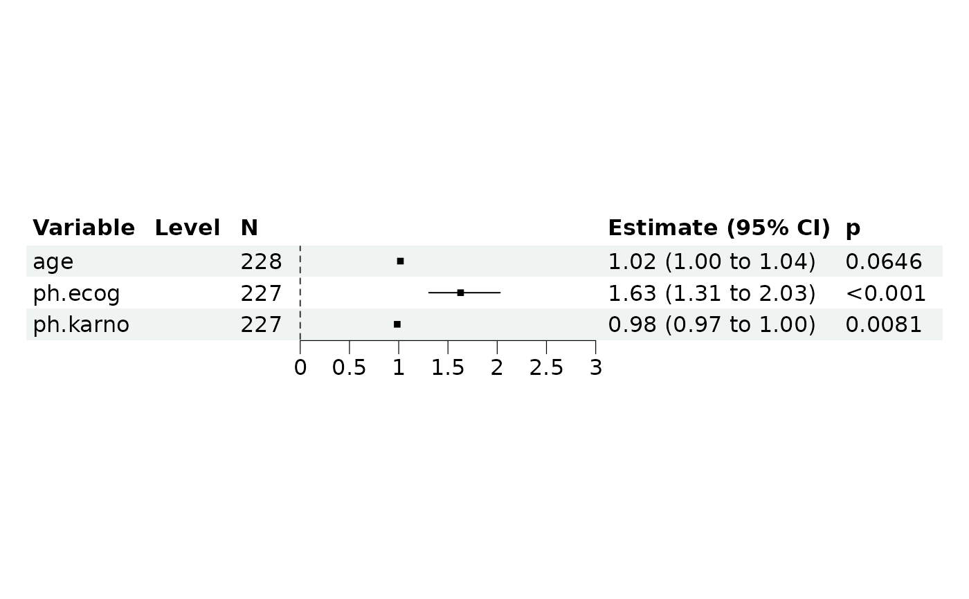
lung <- survival::lung
# Cox-PH regression
ml2 <- REGModelList$new(
  data = lung,
  y = c("time", "status"),
  x = c("age", "ph.ecog", "ph.karno"),
  covars = c("factor(sex)")
)
ml2$build()
ml2$plot_forest()

ml2$plot_connected_risk()
#> please note only continuous focal terms analyzed and visualized


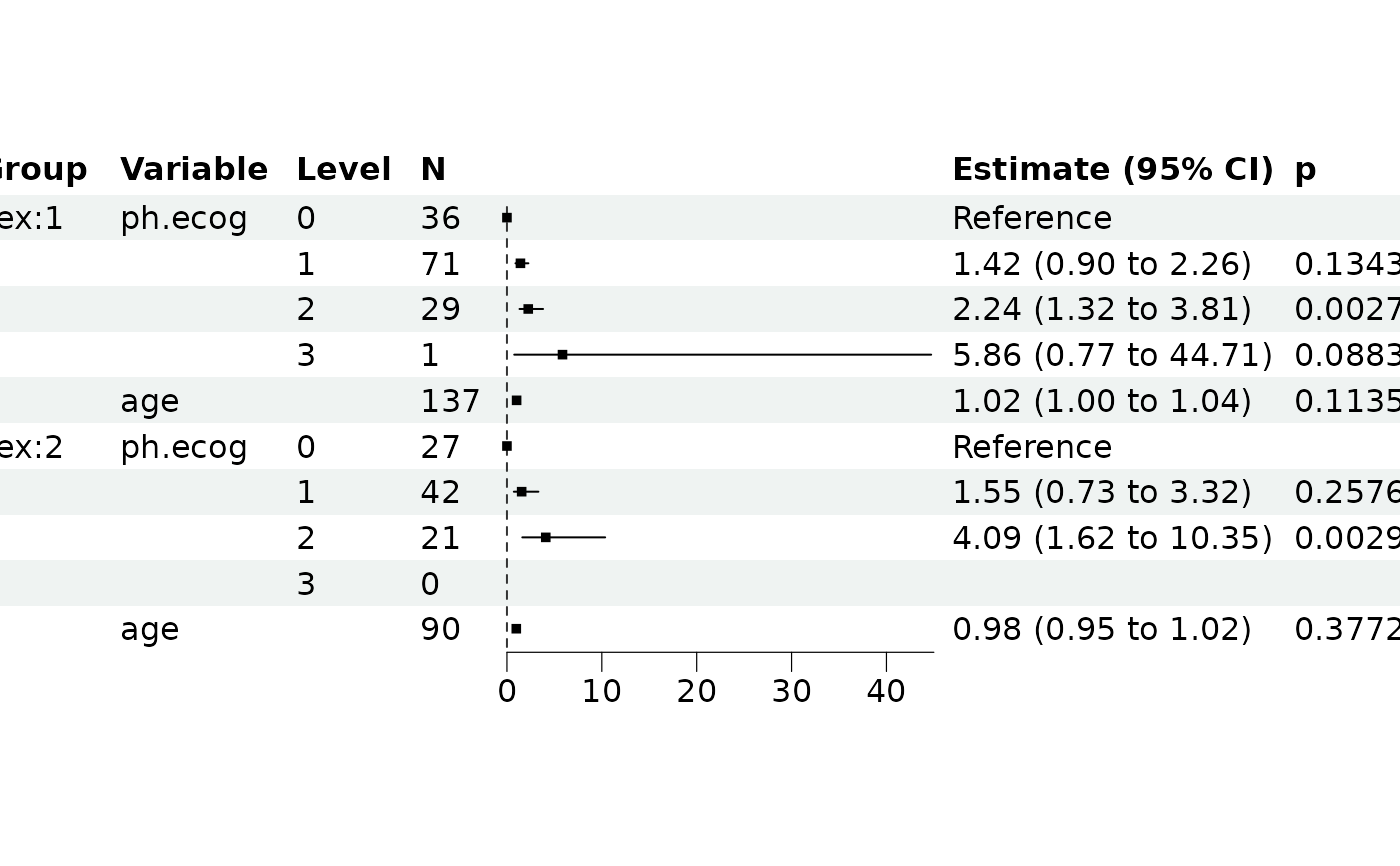
# Group Cox analysis
lung$ph.ecog <- factor(lung$ph.ecog)
ml3 <- REGModelList$new(
  data = lung,
  y = c("time", "status"),
  x = c("ph.ecog"),
  covars = "age", group = "sex"
)
ml3$build()
#> group model data by "sex"
#> Model matrix is rank deficient. Parameters `ph.ecog3` were not
#>   estimable.
ml3$plot_forest()

R6 class representing a list of regression model

Public fields

Methods

Public methods

Method new()

Usage

Arguments

Returns

Method build()

Usage

Arguments

Returns

Method plot_forest()

Usage

Arguments

Method plot_connected_risk()

Usage

Method print()

Usage

Arguments

Method clone()

Usage

Arguments

Examples

Method `new()`

Method `build()`

Method `plot_forest()`

Method `plot_connected_risk()`

Method `print()`

Method `clone()`